
Variance as sensor quality: which sensor to trust
Slide 3 showed that a bell is fixed by its mean and its variance. Now we use the variance to grade sensors. Two friends tell you the time. One checks a good watch and is always within a minute. The other guesses and can be ten minutes off either way. Both are right on average, but you would lean on the first. A sensor whose noise has a small variance is that first friend: its bell is tall and narrow, and its variance is its quality score.
 Lesson 1 · slide 4Sensor quality
- Every measurement is the truth plus noise: z = x + e, where the noise e is a zero-mean Gaussian N(0, σ²).
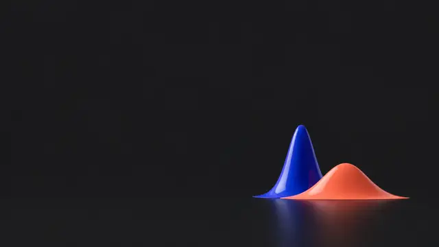
- A good sensor has a small variance: a tall, narrow bell, with readings packed close to the truth.
- A poor sensor has a large variance: a low, wide bell, with readings spread far.
- Averaging n readings divides the variance by n. Combining sensors should lean toward the one with the smaller variance.
The measurement model
Here is the line that sits under every Kalman filter. A sensor measures a true value x and reports a reading z:
Here x is the true value. It is fixed, not random: for a thermometer, the one real temperature in the room. Careful: here x means the fixed true value, not a random variable as on slide 3. Only the noise e is random.
The noise e is a Gaussian with mean 0. "Mean 0" says the sensor has no favourite direction: it is too high as often as it is too low. So on average the readings are right. The variance σ² of that noise is the sensor's quality score: the smaller, the better.
Two sensors, one truth
Picture two thermometers in a 20° room. Both are centred on the truth, so both have mean 20. But sensor 1 has σ = 1° and sensor 2 has σ = 4°.
Sensor 1's bell is tall and narrow: almost every reading is within 2° of the truth. (Each bell holds 100% of the readings, so if it gets narrower it has to get taller.) Sensor 2's bell is low and wide: readings 6° off are not unusual for it. On average both are correct. On any single reading, sensor 1 is far more certain.
That is the whole game. When we combine sensors, we should lean toward the one with the smaller variance. Slide 5 turns that into an exact rule.
Averaging helps, slowly
Can a poor sensor catch up by taking more readings? Yes. The sum of n independent readings has variance n σ², because variances add. The average is that sum divided by n, and dividing by n is scaling by a = 1/n, so the variance is multiplied by a² = 1/n² (slide 3). So:
Taking square roots, σ(average) = σ / √n. So averaging 4 readings halves σ, and averaging 100 readings divides σ by 10.
That works for a parked robot. For a moving drone there is no time to wait, which is why we fuse different sensors instead.
One warning: bias
All of this assumes the noise has mean 0. A thermometer that always reads 2° high has a bias. Averaging cannot remove a bias: a thousand readings that are each 2° high still average 2° high.
Engineers remove bias by calibration, comparing the sensor with a known reference before using it.
Where the numbers come from
A sensor's datasheet usually gives its noise. A phone GPS is good to a few metres. A survey-grade GPS on a mapping drone is good to a couple of centimetres. You can also measure it yourself: hold the sensor still, log a few hundred readings and compute their sample variance s², just as on slide 2. That variance goes straight into the Kalman filter.
A bigger example: three thermometers
Three thermometers hang in a 20° room, with σ = 0.5°, 1° and 2°.
Rank them by variance: smallest first. A self-driving car may carry dozens of sensors, and the filter ranks every one of them the same way.
In the lab
In the lab both sensors start equal (σ = 1), so their bells match. Your job is to make sensor 2 the poor one, like the σ = 4° sensor above, and watch how its bell and its dots change.
Next: we know which sensor to lean on, but not by how much. Slide 5 gives the exact rule for fusing two readings into one better estimate.
Examples
Example 1 · A good and a poor thermometer
Sensor 1 follows N(20, 1), so σ = 1°. Sensor 2 follows N(20, 16), so σ = 4°.
Show solutionHide solution
Same centre. Sensor 2's range is four times as wide, because its σ is four times bigger.
Example 2 · How often within 2°?
You need readings within 2° of the truth. Compare a sensor with σ = 1° and one with σ = 2°.
Show solutionHide solution
Doubling σ turns "almost always" into "about two times in three".
Example 3 · Catching up by averaging
A poor sensor has σ = 4 (variance 16). How many of its readings must you average to match one reading of a sensor with σ = 1 (variance 1)?
Show solutionHide solution
Sixteen readings to match one. Variance grows with σ², so a sensor that is 4 times worse in σ needs 4² = 16 times the readings.
Example 4
Sensor A has variance 0.25. Sensor B has standard deviation 0.4. Which one should you trust more?
Show solutionHide solution
Compare like with like. A: σ = √0.25 = 0.5. B: σ = 0.4, so σ² = 0.16.
B has the smaller variance (0.16 < 0.25), so trust B more.
Example 5
The true temperature is 20°. A sensor with σ = 1° reads 27°. Is that believable? What if the sensor had σ = 4°?
Show solutionHide solution
The miss is 7°. With σ = 1° that is 7σ away: far beyond the 95% range of 18° to 22°. Something is wrong, like a broken sensor or a heater next to it.
With σ = 4° it is 7 / 4 = 1.75σ away, inside the 95% range of 12° to 28°. A normal reading for a poor sensor.
Questions and comments
Stuck on something, or found a mistake? Ask here and I'll answer. You sign in with GitHub.