
The Gaussian bell curve and the 68-95 rule
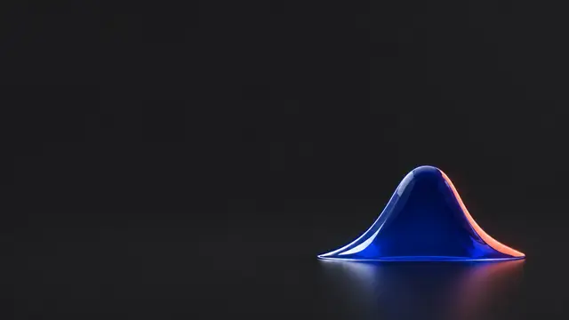
Slide 2 described noise with two numbers, the mean and the variance. Now look at the shape the readings make. Pour sand through a funnel and it piles into a hill: tall in the middle, thin at the edges. Sensor errors pile up the same way, because small errors are common and big ones are rare. That hill is the Gaussian, or bell curve. The mean says where its peak sits and the variance says how wide it is, and those two numbers fix the whole curve.
 Lesson 1 · slide 3The Gaussian
- A Gaussian (normal distribution) N(μ, σ²) is fixed by two numbers: its mean μ (the centre) and its variance σ² (the width).
- About 68% of samples land within ±1σ of the mean, and about 95% within ±2σ.
- Add two independent Gaussians (one tells you nothing about the other) and you get a Gaussian: the means add and the variances add.
- Multiply by a number a and the variance is multiplied by a²: Var(a x) = a² Var(x), where Var(x) means the variance of x.
The bell curve
A distribution says how likely each value of a random variable is. The Gaussian is the most important one for the Kalman filter. We write N(μ, σ²), where N stands for "normal". When a variable x follows this bell we write x ~ N(μ, σ²). Read the ~ as "follows" or "is distributed as".
Its curve has this formula:
Here e = 2.718… is a fixed number, like π, and exp(t) means e to the power t. p(x) is the height of the curve at x: the higher, the more often readings land near x.
It looks scary. Don't be afraid of it: we will almost never plug numbers into it. What matters is what hides inside. Only two numbers appear, μ and σ². The mean μ slides the bell left and right. The variance σ² stretches it wide or squeezes it thin. To model a sensor's noise, that is all we need: where its readings centre and how much they scatter.
The 68-95 rule
Here is a rule of thumb you will use all the time. About 68% of samples fall within one standard deviation of the mean (between μ − σ and μ + σ). About 95% fall within two (between μ − 2σ and μ + 2σ). A reading more than 3σ away is very rare, so it often means something is broken.
So when a datasheet (the maker's spec sheet) says a GPS has σ = 3 m, you know: about 2 readings in 3 land within 3 m of the truth, and almost all within 6 m.
Adding Gaussians
The second reason Gaussians are so handy: they combine with almost no effort. Write Var(x) for the variance of x. Two random variables are independent when one tells you nothing about the other: knowing the error in x gives no hint about the error in y. If x and y are independent, then
And the sum is again a Gaussian. Notice that it is the variances that add, not the standard deviations. Uncertainty piles up: every independent error you add makes the result less certain.
A Gaussian can also describe our own uncertainty. N(30, 4) means "we think the robot is near 30 m, give or take 2 m" (σ = √4 = 2).
Scaling a Gaussian
Multiply a random variable by a number a, and its mean is multiplied by a, but its variance is multiplied by a²:
That makes sense in units. Convert metres to centimetres (a = 100) and the spread in cm is 100 times bigger, so the variance, in cm², is 100² = 10 000 times bigger.
One trap. Say x has variance 4. Add an independent y that also has variance 4: x + y has variance 4 + 4 = 8. But x + x = 2x has variance 2² · 4 = 16, because both copies always err the same way and never cancel. Independence matters.
Put adding and scaling together and you see why averaging works. The average of two independent readings, each N(20, 4), is half their sum: the sum has variance 8, and halving multiplies it by (½)², so the average has variance 2.
A bigger example: four steps in a row
The robot starts at N(30, 4) m and takes 4 steps, each N(5, 1) m, all independent. Add them one at a time, or all at once:
Every step adds 1 to the variance. After 1000 steps it would be 4 + 1000 = 1004, so σ ≈ 31.7 m. Counting steps alone slowly loses track of the robot, which is why lesson 2 adds a GPS.
Why this is all the algebra we need
These few rules are almost the whole toolkit. In lesson 2 the filter's predict step adds the robot's movement to its position: that is "means add, variances add". The correct step fuses two Gaussians: that is slide 5. A drone's tilt (attitude) filter runs these same two moves hundreds of times per second.
Next: a thin bell means readings packed close to the centre, a wide one means they scatter. Slide 4 uses that to decide which of two sensors to trust.
Examples
Example 1 · The 68-95 rule
A thermometer's readings follow N(20, 4), so σ = √4 = 2°.
Show solutionHide solution
A reading of 27° would be 3.5σ away. Possible, but very unlikely.
Example 2 · A robot takes a step
We believe a robot is at N(30, 4) m. Its encoder says it moves N(5, 1) m in one step: we think it moved 5 m, but we are only sure to within about ±1 m. The errors are independent.
Show solutionHide solution
The new position is N(35, 5). The robot moved, and we became a little less sure where it is. This is exactly the predict step of the 1D (one-dimensional: one number, like position along a line) Kalman filter.
Example 3 · Averaging two readings
Two independent readings, each N(20, 4). What is the distribution of their average (x₁ + x₂) / 2?
Show solutionHide solution
The average is N(20, 2): half the variance of one reading. That is why averaging works, and slide 5 will show the same halving when two equal sensors are fused.
Example 4
x ~ N(3, 2) and y ~ N(−1, 5) are independent. Find the distribution of x + y and of x − y.
Show solutionHide solution
x + y: mean 3 + (−1) = 2, variance 2 + 5 = 7. So N(2, 7).
x − y = x + (−1)·y. The mean is 3 − (−1) = 4. The variance of (−1)·y is (−1)² · 5 = 5, so the variance is 2 + 5 = 7 again. So N(4, 7). Subtracting noise still adds variance.
Example 5
A height sensor reads N(2, 0.01) in metres. Write the same reading in centimetres. What is σ in cm?
Show solutionHide solution
Multiply by a = 100. Mean: 2 · 100 = 200 cm. Variance: 0.01 · 100² = 100 cm².
So N(200, 100) and σ = √100 = 10 cm. Check: in metres σ = √0.01 = 0.1 m, which is 10 cm ✓
Questions and comments
Stuck on something, or found a mistake? Ask here and I'll answer. You sign in with GitHub.