
The predict step: move the estimate, grow the variance
Slide 2 ended with two flawed sensors: the encoder is smooth but drifts, and the GPS is centred but jumpy. The Kalman filter uses both, in a loop of two steps. The first is the predict step, and it uses the encoder. Picture standing at the kitchen door, fairly sure where you are, and taking one big step with your eyes closed. You are now about one step further on, and a little less sure than before. The predict step does exactly that to the filter's bell curve: it slides it forward by the encoder's move and makes it a bit wider.
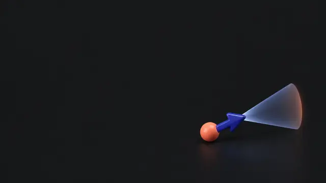 Lesson 2 · slide 3Predict
- The prediction x̂⁻ (say "x-hat minus") is our estimate after the move, before the GPS reading. P⁻ is its variance.
- The mean moves by u, the move the encoder reports (textbooks call u the control input).
- The variance grows by the process noise Q. Predicting never makes you more certain.
- Variances add, not standard deviations: σ⁻ = √(P + Q).
One step in the dark
You know you are at the kitchen door, give or take a little. You close your eyes and take one big step forward. Where are you now? About one step further on. How sure are you? A bit less than before, because the step could have been long or short. That is the whole predict step.
The new words
The filter keeps two numbers about the robot: the estimate x̂ and its variance P. Together they describe a bell curve, N(x̂, P): "the robot is probably near x̂, give or take √P". For example, x̂ = 30 m with P = 4 says "near 30 m, give or take 2 m", and by the 68-95 rule we are about 95% sure it is between 26 and 34 m.
The prediction is written with a small minus: x̂⁻ and P⁻. Read it as "before the measurement". It is where we think the robot is after it moves, before we look at the GPS.
From now on we drop the [n]: x̂ is the estimate from the last step, and x̂⁻ is the new prediction. In the same way, u is the u[n] from slide 1, the move the encoder reports for this step. Textbooks call u the control input, because many robots move by commands ("drive 5 m"). Here it is simply the move the encoder measured. When the encoder measures speed instead, u = speed · Δt, where Δt ("delta t") is the time between steps: a measured speed of 2 m/s with Δt = 0.5 s gives u = 1 m. (In code, Δt is written dt.) The process noise Q is the variance of that move's error. It covers encoder noise, wheel slip and bumps in the floor.
The two equations
The first line moves the mean. The second adds the new doubt to the old doubt. P⁻ is never smaller than P, because Q is never negative. This is the only place the filter's uncertainty grows. With x̂ = 30 m, P = 4, u = 5 m and Q = 1:
Why variances add
The old error and the new step's error are independent. When independent errors add, their variances add. Their σ values do not. With an old σ of 3 m and a step error of σ = 4 m:
The two errors sometimes point in opposite directions and partly cancel, so the total is less than the plain sum.
Predict, predict, predict
If the GPS goes silent, the filter keeps predicting. Each step adds another Q, exactly like dead reckoning on slide 1. Starting from 30 m with P = 4, with u = 5 m and Q = 1 each step:
A bigger example: a robot on a floor
A floor robot moves east and north. For now, treat the two directions as two separate 1D filters, each with its own x̂, P, u and Q. The robot is at 30 m east (P = 4) and 12 m north (P = 2). Each step the encoder says it moved 5 m east (Q = 1) and 2 m south, so −2 m north (Q = 0.5).
Each direction grows its own doubt, by its own Q. A drone does the same for east, north and up, three numbers at once. In real robots the directions are often linked (a wheel slip spoils east and north together). Lesson 3 shows how to handle that.
Where this shows up
A car's navigation keeps your arrow moving in a tunnel by predicting from wheel speed. A drone predicts its next position from its motor commands and its gyro (a sensor that measures how fast it turns) many times a second, between slower GPS readings (called fixes). In both, the predict step is what fills the gaps.
Next: a GPS reading arrives. How far should the filter move toward it, and how much does its doubt shrink? That is the correct step.
Examples
Example 1 · One predict step
The last estimate is x̂ = 30 m with P = 4 (σ = 2 m). The encoder says the robot moved u = 5 m this step, with Q = 1.
Show solutionHide solution
The bell moved 5 m to the right and got a bit wider. We use this prediction again on the next slide.
Example 2 · Three steps in a tunnel
Start from the prediction above, 35 m with P = 5. No GPS for two more steps, same u = 5 and Q = 1.
Show solutionHide solution
P climbs by the same 1 every step. σ climbs a little less each time, because of the square root.
Example 3 · A faster loop
A car drives at 20 m/s, and its filter runs every Δt = 0.1 s. Each step adds Q = 0.01 m².
Show solutionHide solution
A note for later: Q is "per step". If you run the filter twice as often (halve Δt), roughly halve Q too, so one second still adds about 0.1 m².
Example 4
Start with P = 1 and Q = 0.5. How many predict steps, with no GPS, until σ has doubled?
Show solutionHide solution
σ starts at 1, so doubled means σ = 2 and P = 4.
P = 1 + 0.5 · n = 4 gives n = 6 steps.
Example 5
P = 36 (σ = 6 m) and Q = 64 (a step error of σ = 8 m). What is σ⁻ after one predict step? Why is it not 14 m?
Show solutionHide solution
P⁻ = 36 + 64 = 100, so σ⁻ = 10 m.
Variances add, σ values do not. 6 + 8 = 14 would only be right if the two errors always pushed the same way. Independent errors partly cancel.
Questions and comments
Stuck on something, or found a mistake? Ask here and I'll answer. You sign in with GitHub.