
Uncertainty through a Jacobian: σ² ≈ HJ P HJᵀ
Slide 2 gave us the Jacobian: it turns a small move of the robot into a change of the range. Uncertainty is just a cloud of small moves, so the Jacobian carries it too. Picture a tape measure stretched from a wall to a friend. If your friend sways toward or away from the wall, the reading changes. If they sway sideways, it barely moves. The Jacobian says how much of each direction counts, and lesson 3's rule A P Aᵀ does the rest: σᵣ² ≈ HJ P HJᵀ. For an estimate at (3, 4) with σₓ = 0.5 m and σᵧ = 0.8 m, the radar should read 5 m ± 0.71 m.
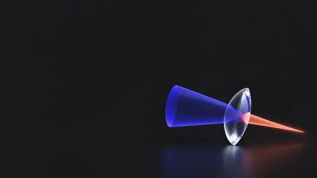 Lesson 4 · slide 3Uncertainty in, out
- On the tangent, the radar is linear, so uncertainty moves through it like through any matrix: HJ P HJᵀ.
- Each slope squared weighs how much that direction's uncertainty reaches the range.
- A correlation in P adds a cross term 2 (∂r/∂x)(∂r/∂y) σₓᵧ, which can raise or lower the result.
- The answer is an approximation: good when the uncertainty is small compared with the distance, poor when it is not.
Only the sway along the line counts
The radar works like the tape measure. Position errors along the line to the radar change the range. Position errors sideways, around the circle, barely change it. The slopes from slide 2, 0.6 for x and 0.8 for y at (3, 4), say how much of each error reaches the reading.
From P to the range's variance
In lesson 3 you pushed a covariance through a matrix: if y = Ax, then the covariance of y is A P Aᵀ. On the tangent the radar behaves like the matrix HJ, so
HJ is one row, so the answer is one number: the variance of the range. When x and y errors are not correlated, P is diagonal and this unpacks into plain numbers: each slope squared, times that direction's variance.
The slopes are squared because variance is in squared units, just like Var(a x) = a² Var(x) in lesson 3. A slope of 0.6 lets through 0.36 of the x variance.
The worked example: 5 m ± 0.71 m
The robot is estimated at x = 3 m, y = 4 m, so r = 5 m and the slopes are 0.6 and 0.8 (slide 2). From here on we look at position only, so the state is just (x, y): we drop the two velocity zeros, HJ = 0.60.8, and P is 2 × 2. (An example below puts velocity back in to show nothing changes.) The position is uncertain by σₓ = 0.5 m and σᵧ = 0.8 m:
In plain words: the radar should read about 5 m, give or take 0.71 m. The y uncertainty dominates. It is bigger, and y also points more along the line to the radar (slope 0.8 against 0.6).
When x and y errors are linked
If P has a covariance σₓᵧ off the diagonal (lesson 3), HJ P HJᵀ picks up one more term: 2 (∂r/∂x)(∂r/∂y) σₓᵧ (as in lesson 3: Var(x + y) = σₓ² + σᵧ² + 2σₓᵧ).
When the errors move together they both push along the line to the radar, and the range gets less certain. When they move opposite ways, the ellipse tilts down to the right. At (3, 4) the circle around the radar runs in the direction (0.8, −0.6), down to the right, so the ellipse lies along the circle, where errors barely change the range.
Checking it with samples
The lab draws 500 possible positions from P, pushes every one through the true radar formula, and compares the spread with the linearised bell. At (3, 4) the samples give a mean near 5.05 and a variance near 0.53, close to 5 and 0.4996. Good enough for a filter.
Now multiply each σ by 4, so each variance by 16 (σₓ = 2, σᵧ = 3.2). That is why the lab line multiplies P by 16. The uncertainty is now comparable to the distance itself.
This is exactly when an EKF starts to go wrong.
Keep reading with the full course
Finish lesson 4 and you will be able to: track a robot from range-only radars with an EKF.
Still locked here:
- The rest of this explanation
- 3 more examples with step-by-step solutions
- Five extra members-only problems with worked solutions
$20 once, lifetime access. Lessons 1 and 2 stay free.
Examples
Example 1 · The numbers from above, exactly
Estimate (3, 4), σₓ = 0.5 m, σᵧ = 0.8 m, HJ = [0.6, 0.8].
Show solutionHide solution
So the range is 5 m ± 0.71 m (one σ). About 95% of readings land within ± 1.41 m.
Example 2 · A correlation in P
Same estimate, but now the x and y errors tend to go together: P = 0.250.20.20.64.
Show solutionHide solution
When x and y errors move together, they both push along the line to the radar, so the range gets less certain. With −0.2 instead, σᵣ² = 0.3076 and σᵣ ≈ 0.555 m.
Questions and comments
Stuck on something, or found a mistake? Ask here and I'll answer. You sign in with GitHub.